Continuous batching, and where the throughput actually goes
A scheduler-level look at continuous batching: why naive static batching wastes most of the GPU, what the arrival-rate math says about queue depth, and the three places real implementations lose the throughput they just won.

Static batching is the first thing anyone builds and the first thing anyone replaces. The reason is easy to state and hard to feel until you watch a profile: in a static batch, every request in the batch finishes when the longest one finishes. A batch of 32 where 31 requests emit 40 tokens and one emits 2,000 spends 98% of its wall time computing on a batch of size one.
Continuous batching fixes the obvious part of this. What it doesn't fix — and what this post is mostly about — is everything downstream of the fix.
The waste, quantified
Take a batch of requests where request generates tokens. Static batching runs decode steps and the batch occupancy at step is the number of requests still alive:
Average utilization over the life of the batch is therefore the mean output length over the max:
Output lengths in real traffic are heavy-tailed, so grows with while doesn't. Utilization falls as you increase batch size, which is the opposite of what batching is supposed to do. For a Pareto-ish length distribution with and a p99 of 2,000, a batch of 64 lands near .
Continuous batching replaces a finished request's slot immediately, so occupancy stays near the slot limit and stops depending on the tail.
What a step actually looks like
The scheduler loop is small enough to write down. Each iteration it picks a set of running sequences, optionally admits new ones, and issues exactly one forward pass:
def step(self) -> list[Output]:
    # Evict before admitting: a preempted sequence frees blocks that an
    # admission may need in this same iteration.
    self._preempt_if_over_budget()

    admitted = self._admit_waiting()          # prefill candidates
    running = self.running + admitted

    if not running:
        return []

    # One fused forward pass over prefill + decode tokens.
    batch = self._build_batch(running)
    logits = self.model.forward(batch)

    outputs = []
    for seq, token in zip(running, self.sampler(logits)):
        seq.append(token)
        if seq.is_finished():
            self.kv_cache.free(seq.block_ids)   # slot reopens immediately
            outputs.append(seq.finalize())
        else:
            self.running_next.append(seq)

    self.running = self.running_next
    self.running_next = []
    return outputs
The interesting line is self.kv_cache.free(...). Everything continuous batching
buys you comes from that call happening at step granularity instead of batch
granularity.
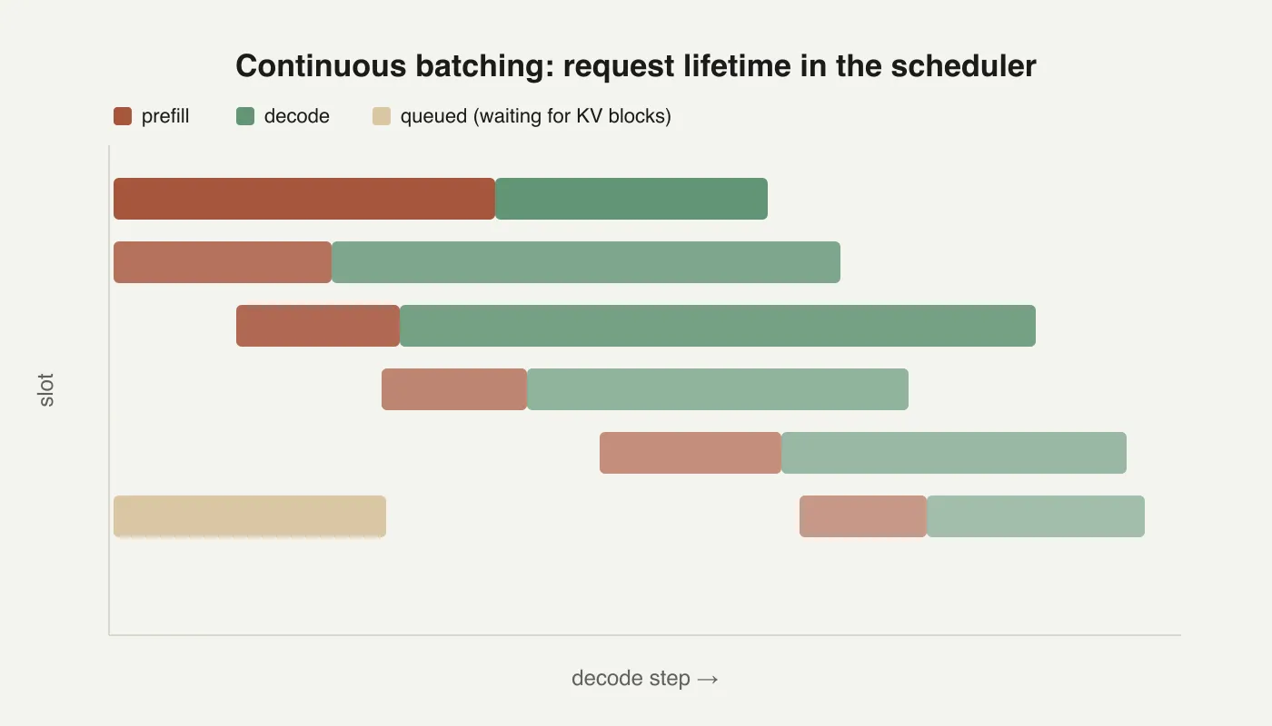
Drawn this way the mechanism is obvious: the gaps a static batch would leave on the right-hand side of every short request are backfilled by whatever is waiting.
Where the throughput leaks back out
Three places, in rough order of how much they cost.
1. Prefill stalls the decode stream
A fused batch mixes a long prefill with many short decodes. Prefill is compute- bound and scales with the square of sequence length in attention; decode is memory-bound and scales with batch size. Put a 4,000-token prefill in the same forward pass as 60 decodes and every one of those decodes waits on the prefill's GEMMs.
Chunked prefill splits the prompt into fixed-size pieces so any single step has a bounded compute budget:
| Strategy | p50 TPOT | p99 TPOT | Throughput |
|---|---|---|---|
| Fused, unbounded prefill | 24 ms | 310 ms | 1.00× |
| Chunked prefill, 512 tokens | 27 ms | 61 ms | 0.97× |
| Prefill/decode disaggregated | 21 ms | 44 ms | 1.11× |
The p99 column is the reason anyone bothers. Throughput barely moves; tail latency moves by 5×.
2. The KV cache runs out before the slots do
Slot count is not the real admission limit — KV blocks are. A sequence at length with KV heads, head dimension , layers, and 2 bytes per element occupies
per sequence, for keys and values together. With , , , that is 512 KiB per 1,000 tokens per sequence. Eighty concurrent sequences at 4,000 tokens each is 16 GiB of cache alone, before weights or activations.
So the admission test is a memory test, and it has to be predictive: admitting a sequence you will have to preempt three steps later costs you the prefill twice.
3. Python gets in the way
At 60 concurrent sequences and 25 ms per step, the scheduler has ~400 μs of CPU budget per sequence per step to build the batch, update block tables, sample, and detokenize. Naive per-sequence Python work blows through that. The usual fixes:
- Keep block tables as preallocated tensors, not lists of lists.
- Batch detokenization and run it off the critical path.
- Overlap the next step's CPU preparation with the current step's GPU execution.
- Cache the sampling metadata that doesn't change between steps.
Reading a profile honestly
Two numbers decide whether you have a scheduling problem or a kernel problem:
- Step occupancy. Average running-sequence count divided by the slot limit. Below ~0.8 under sustained load, the admission path is the problem.
- GPU idle fraction between steps. More than a few percent and the CPU-side scheduler is the bottleneck, not the model.
Both are cheap to instrument and both are routinely skipped in favour of staring at kernel timings that were never the limiting factor.
Further reading
The vLLM paper1 is the canonical treatment of paged KV management, and Orca2 introduced iteration-level scheduling, which is continuous batching by another name.